This Is Not the Anonymization You're Looking For

Or, how to turn a hackathon into a hands on privacy lab

What happens when a data science competition releases two “anonymous” datasets on consecutive days, changes every identifier, and still leaves the underlying structure intact?

For a team at ITADATAHack 2026, that question became as interesting as the recommendation problem itself. K!nd4SUS president Samuele Manclossi, student representative Riccardo Pasquino, and Raffaele Valendino formed the independent team MLoops and discovered that the two tasks could be connected. By treating playlists and artists as structural fingerprints, MLoops recovered most of the hidden correspondence between the releases and used it to improve the second task.

This is the story of the competition, the attack, and the broader privacy lesson behind it.

A music recommender in two acts

ITADATAHack 2026 was the fourth edition of the national data science competition organized by the CINI Data Science Lab and hosted by the University of Bari as part of the ITADATA 2026 conference. The online phase ran from 09:00 on 16 October to 21:00 on 17 October 2026; the final was scheduled for 10 November in Bari, with remote participation available to finalists. Teams consisted of two or three eligible students or recent graduates. [1]

The challenge was to build a music recommendation system from a synthetic dataset derived from public data. Each row represented a playlist and each column an artist. A cell contained the multiplicity of that artist in the playlist - in plain terms, how many tracks by that artist the playlist contained. Names were replaced by identifiers such as P123 for playlists and A456 for artists.

The competition was divided into two tasks of increasing complexity:

• Task 1, open for the first 24 hours, provided 4,170 labelled training playlists and 1,167 test playlists. Participants saw counts for 2,990 non target artists and had to predict the presence or absence of ten hidden target artists. The metric was the sample averaged F1 score. [7]

• Task 2, open for the final 12 hours, provided 4,144 labelled training playlists and 1,037 test playlists. This time there were 2,970 visible artists and 30 targets. For every playlist, teams had to select exactly five target artists in the hope of covering the ground truth top three by multiplicity, including any ties. [8]

Each team worked through a shared HPC4AI account and JupyterHub environment. A valid submission required both predictions and the notebook that produced them. Scores appeared on a live leaderboard, only a team’s two best submissions were retained, and at least two minutes had to pass between submissions. After the online phase, the jury would inspect the notebooks of the top 15 teams before choosing the finalists. [1]

MLoops was the team which performed the attack. It stopped submitting at 18:00 on 17 October, three hours before the official closing time. At that moment Task 2 was still live and the independent team was in second place with a score of 0.9293, behind Trigon at 0.9487 and ahead of Happy Angels at 0.7215. The image records the situation when the team stopped playing, not the final standings. [11]

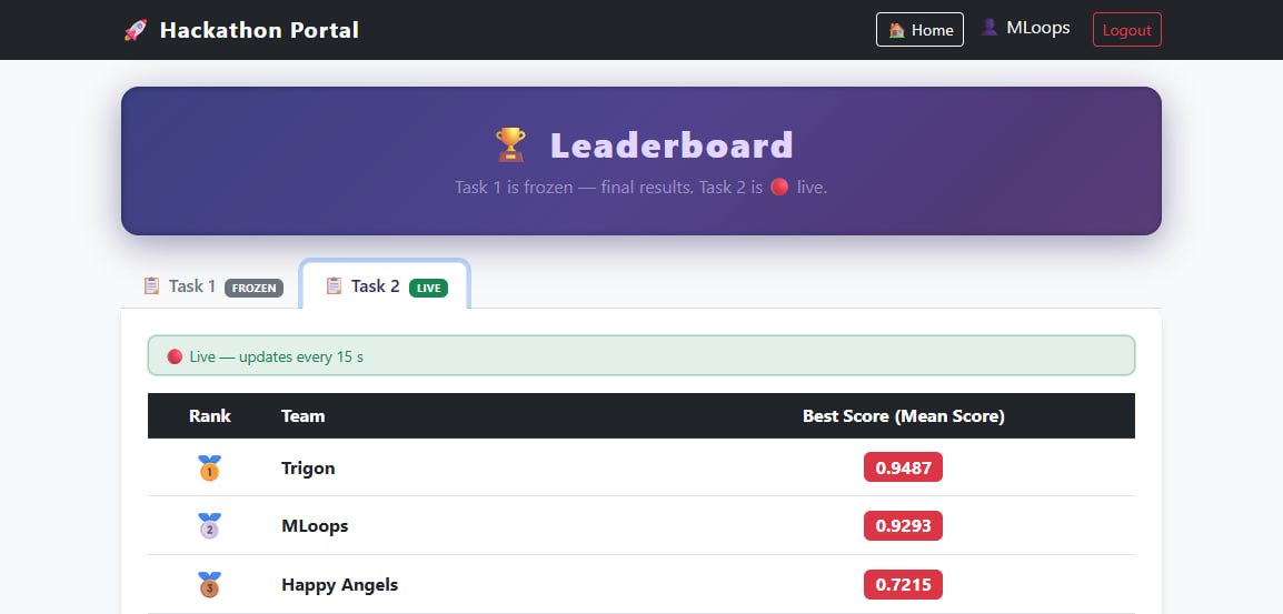
Figure 1. At 18:00, when MLoops stopped submitting, it held second place with 0.9293. Because Task 2 was still live, this is a snapshot of the position the team left behind rather than a final ranking.

At first sight, Task 2 was simply a harder recommender problem. But its relationship with Task 1 created another route.

What is a linking attack?

A linking attack combines two or more datasets to discover which records refer to the same underlying entity. Removing names is not always enough: dates, locations, preferences, relationships, counts, and other quasi identifiers can form a distinctive signature. NIST explicitly warns that deidentified data can sometimes be reidentified when it is combined with auxiliary information. [2]

Imagine two anonymous shopping datasets. One says that customer X17 bought coffee, a rare camera lens, and three train tickets on particular days. The other calls its customers by different codes, but Q82 shows the same unusual pattern. Neither dataset contains a name, yet the pattern strongly suggests that X17 and Q82 are the same customer. If one release contains a field hidden by the other, the link transfers that information across the boundary.

The ITADATAHack case follows the same logic, with two important qualifications. First, the goal was to match records and artist columns across the two competition releases - not to recover identifiers through a direct key. Second, the competition data was synthetic. The attack did not identify real Spotify listeners or reveal the real names of artists. It demonstrated that the supposedly separate pseudonymous releases were linkable and that this link leaked information relevant to Task 2.

We have seen this pattern before

Linking attacks are not a new corner case. Several incidents have become landmarks in privacy engineering:

• In the 1990s, Latanya Sweeney linked supposedly anonymous Massachusetts medical records with public voter registration data using ZIP code, birth date, and sex. This singled out the medical record of then governor William Weld. The episode helped motivate formal privacy models such as k anonymity, which was developed jointly by Sweeney and Pierangela Samarati. [3] [6]

• In 2006, AOL released millions of search queries under numeric user identifiers. Reporters connected the searches of user 4417749 - including names, places, and personal concerns - to Thelma Arnold, demonstrating that replacing a name with a number does not make a detailed behavioural history anonymous. [4]

• In 2008, Arvind Narayanan and Vitaly Shmatikov showed that sparse movie rating histories in the Netflix Prize dataset could be linked to public IMDb ratings. A small amount of approximate background knowledge could be enough to locate a subscriber’s record and expose other ratings. [5]

These cases differ in data type and consequence, but the mechanism is consistent: data with many dimensions contains rare combinations, and rare combinations make excellent fingerprints.

How we linked the two ITADATAHack releases

The two tasks each described a universe of 3,000 artists, but divided it differently: Task 1 exposed 2,990 artists and hid ten as labels; Task 2 exposed 2,970 and hid 30. Both playlist and artist identifiers had been reassigned, so there was no shared name to join on. The values themselves, however, preserved enough common structure. [7] [8]

It helps to view each release as a sparse matrix. Playlists are rows, artists are columns, and multiplicities are cells. Renaming and reordering the rows and columns changes the coordinates, but it does not change the underlying patterns. If two rows represent the same playlist, they still contain the same collection of multiplicities in a different column order. If two columns represent the same artist, they contain the same multiplicities when read across correctly linked playlists.

This creates a feedback loop. A few playlist links make artist links possible. Those artist links create much stronger playlist signatures, which reveal more playlist links. The larger set of playlists then reveals more artists.

1. Find a rough orientation

The first step compared the cooccurrence graph of Task 2’s 30 target labels with a graph built from the 30 most prevalent Task 1 input artists. Each graph recorded which candidates tended to appear in the same playlists. A quadratic assignment searched for a permutation that made those neighbourhoods resemble each other.

This produced a working orientation, not a final identity map. The audit later found that this graph seed agreed with the stronger final mapping for just 7 of the 30 targets. A plausible statistical alignment can help a bootstrap process begin, but it is not proof. [9]

2. Seed playlist matches with permutation invariant fingerprints

Renaming artists changes the order of a playlist’s columns, but it does not change the histogram of its nonzero counts. A playlist with, for example, six artists appearing once, two appearing twice, and one appearing four times keeps the count pattern {1: 6, 2: 2, 4: 1} under every column permutation.

The two releases first had to be made comparable. On the Task 1 side, the code temporarily removed the 30 artists provisionally identified as Task 2 targets, then appended the ten Task 1 presence labels. This produced a 2,970 position view to compare with Task 2’s 2,970 input columns. The appended labels are binary rather than full counts, so requiring exact histogram agreement was deliberately conservative.

For every eligible Task 1 training row, the code used the provisional artist alignment to reconstruct a tentative Task 2 target pattern. It considered only Task 2 training rows with that same pattern. Within this smaller candidate set, it compared the count histograms and required the best candidate to match exactly. It also required the next best candidate to be at least three histogram edits away. These filters yielded 32 conservative playlist pairs, the small foothold needed for the next stage. [9]

3. Alternate between rows and columns

Once playlists had been paired, each candidate artist column still visible as counts could be represented by its vector over those pairs. Suppose a Task 1 column has counts [2, 0, 1] on three linked playlists. If exactly one Task 2 column has the same vector on the corresponding three playlists, the two columns are strong candidates for the same artist. The implementation accepted only vectors that were unique on both sides and had enough nonzero support.

The direction was then reversed. The matched artist columns were put into a common order, so each playlist could be represented by its values on known artists. If a Task 1 row and a Task 2 row had the same signature, that signature occurred only once, and it contained enough nonzero observations, the rows were linked. Every accepted link also had to preserve a one to one mapping, so two rows or columns could not claim the same partner.

In compact form, each round did the following:

1. Read artist columns across the known playlist pairs.
2. Link the unique columns whose count vectors were exactly equal.
3. Read playlists across those newly linked artist columns.
4. Link the unique rows whose signatures were exactly equal.
5. Repeat with the larger evidence set.

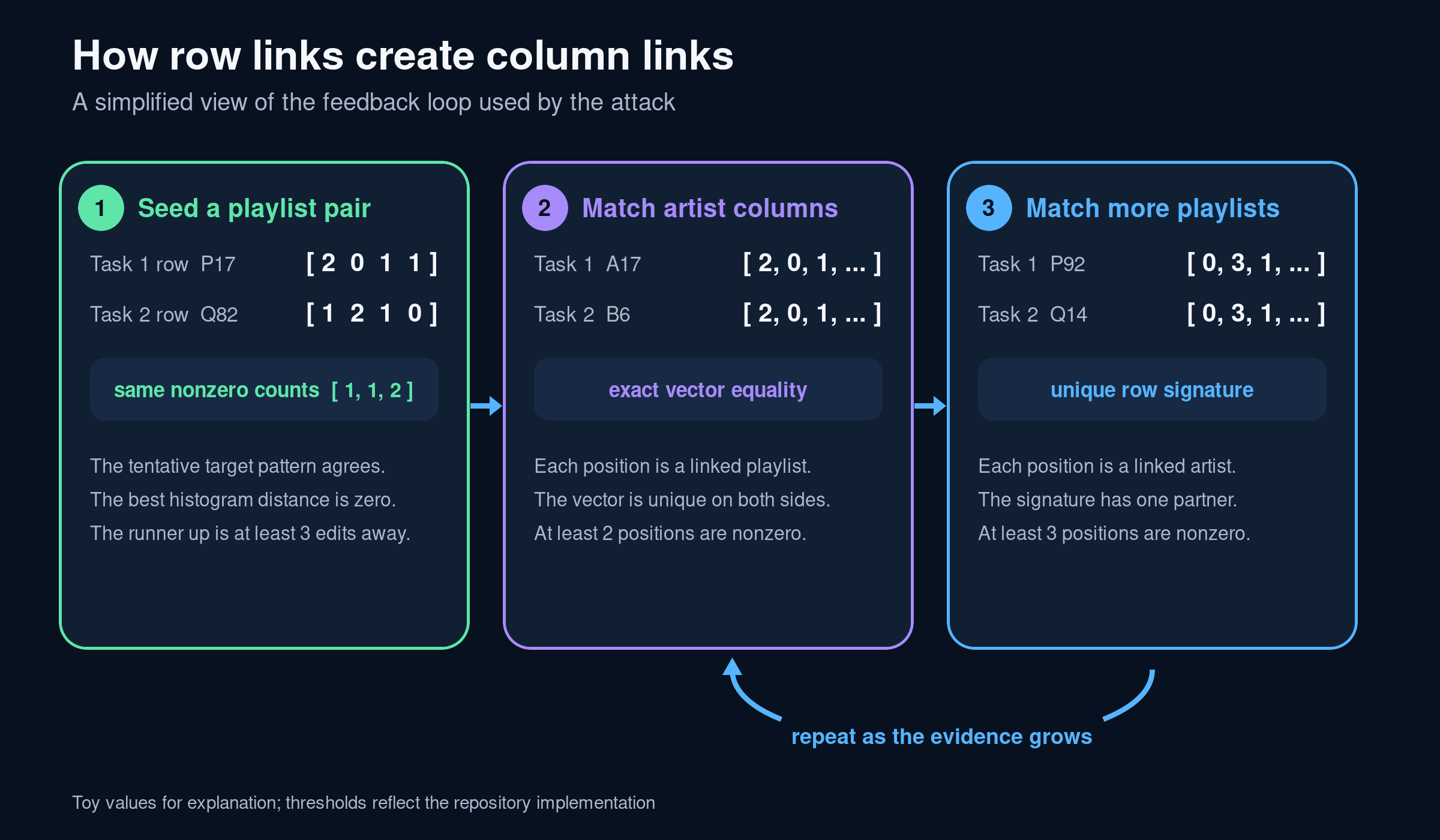
Figure 2. The attack’s engine was reciprocal evidence: a playlist match created a coordinate system for comparing artists, and every artist match made the next playlist signature more distinctive. The real implementation required unique signatures, minimum support, and a one to one mapping at each step.

Repeating this cycle between rows and columns caused the linkage to snowball:

Initial invariant seeds: 32 linked playlists and 0 matched artist columns.

After labelled data iterations: 177 linked playlists and 362 matched artist columns.

After the first iteration over all rows: 3,652 linked playlists and 366 matched artist columns.

Final convergence: 4,123 linked playlists and 2,828 matched artist columns. [9]

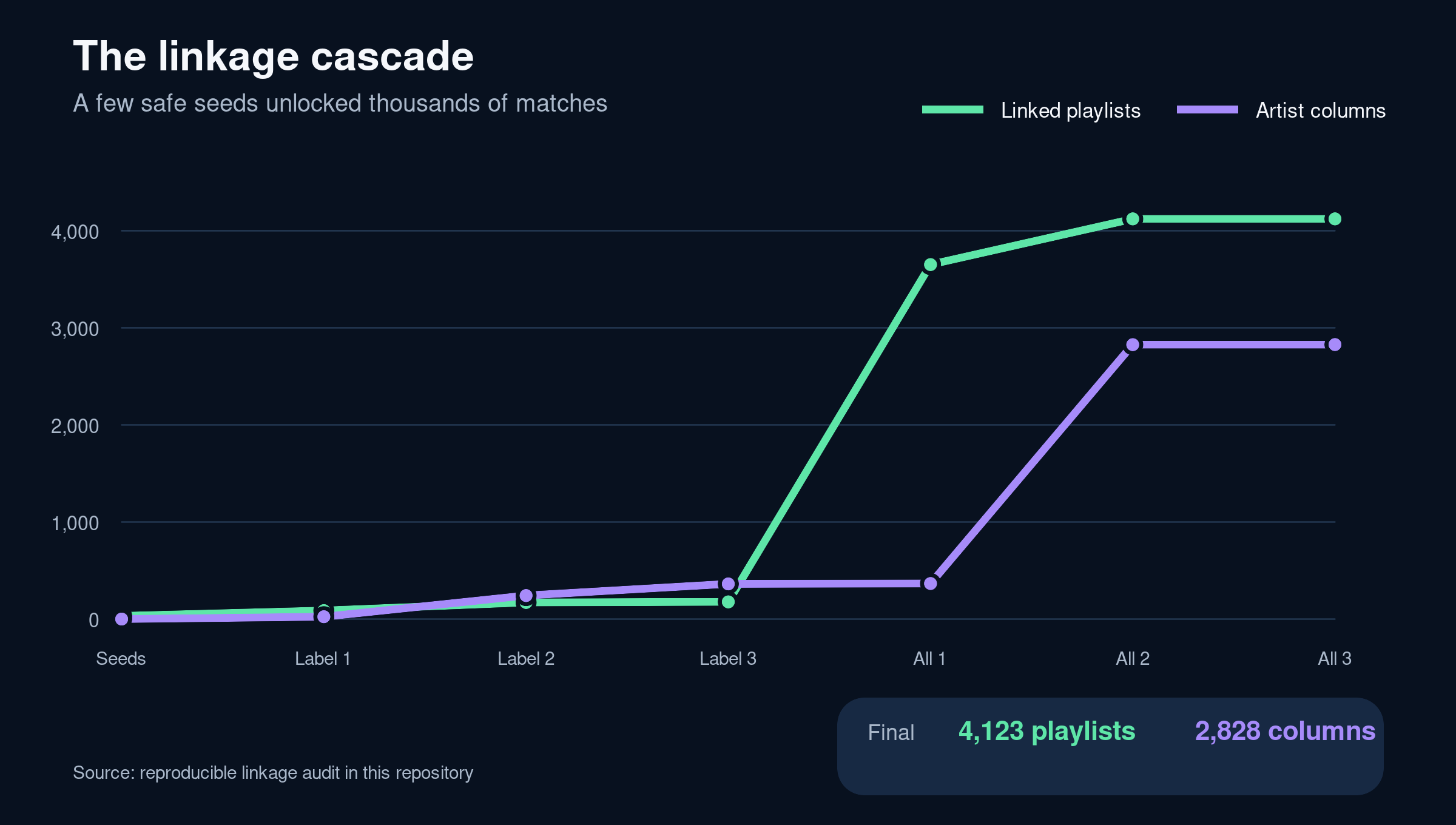
Figure 3. This is the privacy failure in one curve: 32 invariant playlist seeds were enough to bootstrap 4,123 playlist links and 2,828 exact artist column links.

The crucial lesson is that a tiny number of high confidence links can unlock much more of a dataset when the same sparse structure is released twice.

4. Recover the hidden targets

With thousands of playlist pairs available, the 30 Task 2 targets could be mapped more directly. A positive Task 2 target label says that its artist is among that playlist’s top three targets. Therefore, the corresponding Task 1 artist must at least be present in the linked Task 1 playlist. For every possible target and Task 1 artist pairing, the code counted violations of this containment rule, then solved a global one to one assignment that minimized the total violations.

Containment identifies candidates, while the original counts provide a stronger check. The code used the selected Task 1 artists’ multiplicities to reconstruct Task 2’s complete top three with ties labels. Across 3,267 validation playlists and 30 target cells each, the reconstruction differed in only 20 cells, an error rate of about 0.0204%. [9]

The ten artists that appeared only as Task 1 labels were handled by matching their binary presence vectors to Task 2 input columns over already linked playlists.

5. Mark inference as inference

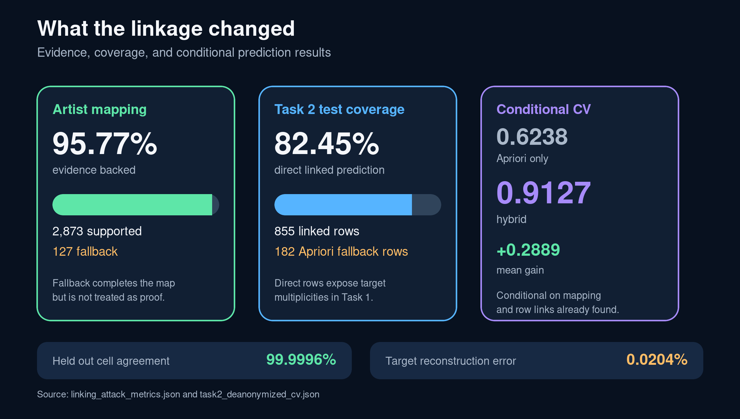
The final map was a bijection covering all 3,000 artists, but not every entry had equal evidential strength. The audit classified 2,873 mappings, or 95.77%, as evidence backed exact or near exact links. The remaining 127 low support artists were assigned by comparing their relationships to strong “anchor” artists and solving another global one to one assignment.

Those 127 are explicitly marked as fallback mappings. A bijection is internally consistent, but it is not ground truth, and the audit does not pretend otherwise. Held out checks were nevertheless strong: 99.225% of discovered artist links reproduced an entire held out column exactly, while cell level agreement was 99.9996%. [9]

From linkage to recommendations

The link made part of Task 2 much easier. For a linked Task 2 test playlist, the matching Task 1 playlist was known. The Task 2 targets had also been mapped to Task 1 columns, where their exact multiplicities were visible. Instead of estimating which targets belonged near the top, the system could rank those observed counts directly and produce the required five selections.

This direct route covered 855 of the 1,037 Task 2 test playlists, or 82.45%. For the remaining 182, the team used an Apriori style fallback based on count thresholds and frequent artist pair rules. [10]

In five fold conditional cross validation, the Apriori only method averaged 0.6238, while the hybrid of direct linked predictions and Apriori fallback averaged 0.9127, a gain of 0.2889 under the official Task 2 metric. “Conditional” matters here: the folds evaluated predictions given the already recovered mapping and row links; they did not rerun the entire discovery attack independently inside every fold. These figures therefore measure the value of the linkage once obtained, not a fully independent evaluation of the complete discovery process. [10]

Figure 4. Linkage changed the nature of the recommendation task: 82.45% of the test playlists became direct lookups, while 127 artist identities and 182 playlists still required explicitly marked fallback inference.

Anonymization is a property of a release and its context

Changing IDs protected the literal lookup table, but it did not erase the relationships encoded by the data. Sparse playlists retained their count fingerprints. Artists retained their cooccurrence patterns. Releasing a second view of overlapping entities supplied the auxiliary information that the first release lacked.

That is the broader lesson for challenge designers and data publishers:

• assess all planned releases together, not one file at a time;
• treat stable patterns across many dimensions as potential identifiers;
• test for linkage across train and test splits and successive tasks before publication;
• minimize overlap that is not necessary for the challenge;
• use measurable privacy protections and adversarial reidentification testing instead of relying on renamed columns alone. [2]

For MLoops, ITADATAHack 2026 became more than a recommender system contest. The independent team’s work offered K!nd4SUS readers a compact demonstration of an old security principle: identifiers are not the only things that identify. Sometimes the shape of the data says more than its name.

Sources

[1] Official ITADATAHack 2026 event page, CINI Data Science Lab and ITADATA.

[2] Simson L. Garfinkel, NISTIR 8053 on removing identifiers from personal information, National Institute of Standards and Technology, 2015.

[3] Lynne Lamberg, Confidentiality and Privacy of Electronic Medical Records, JAMA, 2001; and Latanya Sweeney, A Model for Protecting Privacy with k Anonymity, 2002.

[4] Michael Barbaro and Tom Zeller Jr., A Face Is Exposed for AOL Searcher No. 4417749, The New York Times, 2006. A verifiable archived copy is preserved by the Electronic Frontier Foundation.

[5] Arvind Narayanan and Vitaly Shmatikov, the 2008 IEEE paper on robust deanonymization of large sparse datasets, which documents the Netflix Prize attack.

[6] Pierangela Samarati and Latanya Sweeney, their joint 1998 SRI technical report on k anonymity.

[7] Official Task 1 description, task1_description.pdf, supplied by the competition organizers.

[8] Official Task 2 description, task2_description.pdf, supplied by the competition organizers.

[9] Reproducible linking attack metrics, linking_attack_metrics.json, generated by this_is_not_the_anonymization_youre_looking_for_v2.ipynb.

[10] Conditional Task 2 evaluation report, task2_deanonymized_cv.json, generated by the repository evaluation notebook.

[11] Task 2 live scoreboard snapshot at 18:00, scoreboard.jpg, preserved by the independent MLoops team during the competition.

Link to the repo will be available soon.